boston_housing

Udacity Machine Learning Nano degree Program. Project Predicting House prices in Boston

Project maintained by prateekiiest Hosted on GitHub Pages — Theme by mattgraham

Predicting House Prices in Boston

Project 1: Model Evaluation & Validation

Predicting Boston Housing Prices

This document describes the implementation of a Machine Learning regressor that is capable of predicting Boston housing prices. The data used here is loaded in (sklearn.datasets.load_boston) and comes from the StatLib library which is maintained at Carnegie Mellon University. You can find more information on this dataset from the UCI Machine Learning Repository page.

Statistical analysis

Total number of houses: 506
Total number of features: 13
Minimum house price: 5.0
Maximum house price: 50.0
Mean house price: 22.533
Median house price: 21.2
Standard deviation of house price: 9.188

Evaluating model performance

The problem of predicting the housing prices is not a classification problem since the numbers changing with the time. So it is a Regression problem and uses regression problem’s evaluation metrics for model evaluation.

Measures of model performance

I think Mean Squared Error(MSE) is the most appropriate metric to use based on the following reasons:

Predicting housing price problem is a regression problem since prices changes over time. So we cannot use Classification metrics such as ‘Accuracy’, ‘Precision’, ‘Recall’ and ‘F1 Score’. Hence We need to choose between ‘MSE’ and ‘MAE’.
Between ‘MSE’ and ‘MAE’ both can work well with this problem but I would rather use ‘MSE’ due ti its properties. ‘MSE’ penalizes larger errors more than smaller ones( since it is squarifies the absolute error so 0.2 will calc for 0.04 but 20 will be 40) and also it is a differentaible function.

Splitting the data

Learning the parameters of a prediction function and testing it on the same data is a methodological mistake: a model that would just repeat the labels of the samples that it has just seen would have a perfect score but would fail to predict anything useful on yet-unseen data. This situation is called overfitting. To avoid it, it is common practice when performing a (supervised) machine learning experiment to hold out part of the available data as a test set X_test, y_test.(*)

Hence to properly evaluate the model, the data we have must be split into two sets: a training set and a testing set to be able to:

Give estimate on performance on independant datasets
Serves as a check for overfitting

(*) Scikitlearn documentation.

Cross-Validation

Even if we split the data, our knowledge while tuning a model’s parameters can add biases to the model, which can still be overfit to the test data. Therefore, ideally we need a third set the model has never seen to truly evaluate its performance. The drawback of splitting the data into a third set for model validation is that we lose valuable data that could be used to better tune the model.

An alternative to separating the data is to use cross-validation. Cross-validation is a way to predict the fit of a model to a hypothetical validation set when such a set is not explicitly available. There is a variety of ways in which cross-validation can be done. These methods can be divided into two groups: exhaustive cross-validation, and non-exhaustive cross-validation. Exhaustive methods are methods which learn and test on all possible ways to divide the original data into a training and a testing set. As such, these methods can take a while to compute, especially as the amount of data increases. Non-exhaustive methods, as the name says, do not compute all ways of splitting the data.

K-fold cross-validation in an example of exhaustice method, which consists of randomly partitioning the data into k equal sized subsets. Of these, one subset becomes the validation set, while the other sets are used for training the model, and the process is executed k times, one for each validation subset. The performance of the model, then, is the average of the performance of model in each of the k executions. This method is attractive because all data points are used in the overall process, with each point used only once for validation.

Grid Search: Searching for estimator parameters

Machine learning models are basically mathematical functions that represent the relationship between different aspects of data. Models can have parameters some can be learnt during the trainig phase ans some other which called hyperparameters must be specified outside the training procedures such as decision trees depth ot number of leaves. This type of hyperparameter controls the capacity of the model, i.e., how flexible the model is, how many degrees of freedom it has in fitting the data. Proper control of model capacity can prevent overfitting, which happens when the model is too flexible, and the training process adapts too much to the training data, thereby losing predictive accuracy on new test data. So a proper setting of the hyperparameters is important.

Grid search is one of the algorithms used for tuning hyperparameters; true to its name, picks out a grid of hyperparameter values, evaluates every one of them, and returns the winner. For example, if the hyperparameter is the number of leaves in a decision tree, then the grid could be 10, 20, 30, …, 100. For regularization parameters. Some guess work is necessary to specify the minimum and maximum values. So sometimes people run a small grid, see if the optimum lies at either end point, and then expand the grid in that direction. This is called manual grid search.

Grid search is dead simple to set up and trivial to parallelize. It is the most expensive method in terms of total computation time. However, if run in parallel, it is fast in terms of wall clock time.

Analyzing Model Performance

Up to this point we’ve been describing the techniques used: MSE as performance metric, splitting the data between training and test, $k$-fold cross-validation for validation and an exhaustive grid search for finding the best parameters. In this section we will analyse the model constructed.

The model we built is a decision tree regressor in which we varied the maximum tree depth by passing the max_depth argument to sklearn’s DecisionTreeRegressor.

  ``` # Create four different models based on max_depth
      for k, depth in enumerate([1,2,3,4,5,6,7,8,9,10]):

    for i, s in enumerate(sizes):

        # Setup a decision tree regressor so that it learns a tree with max_depth = depth
        regressor = DecisionTreeRegressor(max_depth = depth)

        # Fit the learner to the training data
        regressor.fit(X_train[:s], y_train[:s])

        # Find the performance on the training set
        train_err[i] = performance_metric(y_train[:s], regressor.predict(X_train[:s]))

        # Find the performance on the testing set
        test_err[i] = performance_metric(y_test, regressor.predict(X_test))```

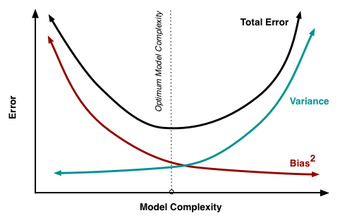
Bias and Variance

We have plotted 10 different graphs of decision trees performance. Based on our analysis on the graphs we have found an important relationship: The more we increase the tree depth, the more we reduce the training error, which goes down to practically zero. The training error, though, seems to find its best values around depths 6 & 5, and then starts to increase with the maximum tree depth. 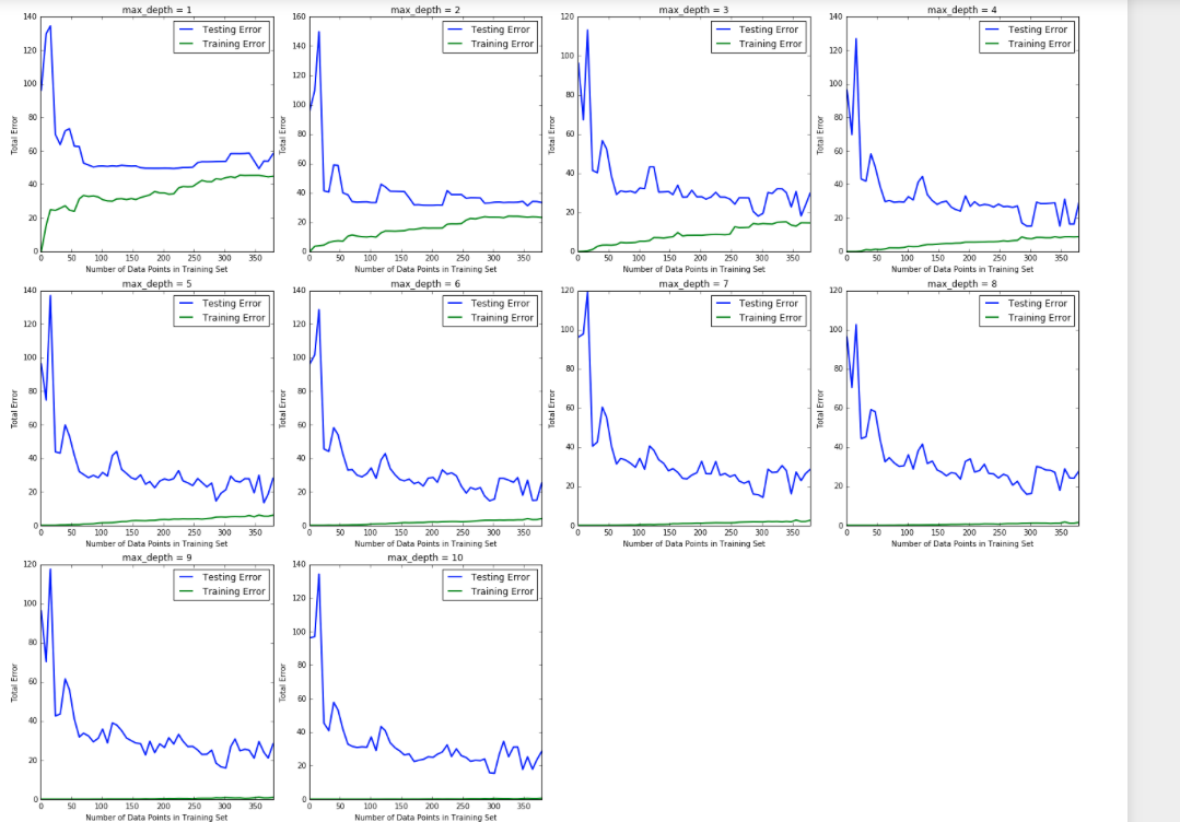Alt text When max depth was 1, the model was suffering from high bias. The model was performing poorly not only on the test set, but also on the training set. This means that no matter how much data we give it, it does not capture the relationships and patterns in the data which can help us improve predictive performance. On the other hand, when the max depth was 10, the model was suffering from overfitting. In this case, the training error was virtually nil. However, the test error was still significant. The model, at this point, has “memorized” the training set such that the training error is low, but cannot generalize well enough to do well with unseen data.

Model Complexity

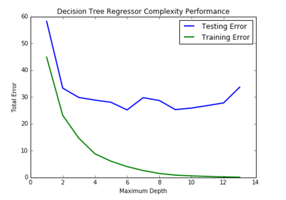Alt text As max depth increases training errors decreases from 45 at the beginning to nearly zero but the testing error has a drastic desrease at the beginning but it will stay steady between 30 to 40. This indicates the variance is steady and model is not generalized enough since there are some drastic increases in max depth 6 and 12. The (max_depth=5) appears to yield the model that will generalize the best.Which is confirmed by calling the best_params_member of GridSearchCV which gives values in the range [5, 6] with high frequency, and sometimes 4, or 7. This is due to the random sampling in the way cross-validation is done. So we should choose the least complex model that explains the data, and I’d go with 5 here.

Alt text

Results

Check here - Udacity Reviews

Installation

This project requires Python 2.7 and the following Python libraries installed:

You will also need to have software installed to run and execute an iPython Notebook

Udacity recommends our students install Anaconda, i pre-packaged Python distribution that contains all of the necessary libraries and software for this project.

Run

In a terminal or command window, navigate to the top-level project directory boston_housing/ (that contains this README) and run one of the following commands:

ipython notebook boston_housing.ipynb

This will open the iPython Notebook software and project file in your browser.

Contribution

There is isn’t much to contribute to, but still if you want to suggest a new algorithm(a better one whuch might give a better accuracy) then you are welcome. First Create an Issue and state your contribution.If approved you are welcome to send a PR.